Note
Click here to download the full example code
Pitch Visualisations
First we import the Pitch classes and matplotlib
import matplotlib.pyplot as plt

from mplsoccer import Pitch, VerticalPitch
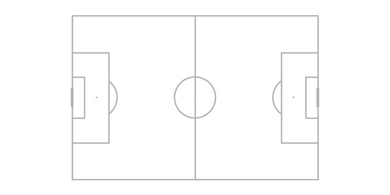
Draw a pitch on a new axis
Let’s plot on a new axis first.
pitch = Pitch()
# specifying figure size (width, height)
fig, ax = pitch.draw(figsize=(8, 4))
Draw on an existing axis
mplsoccer also plays nicely with other matplotlib figures. To draw a pitch on an
existing matplotlib axis specify an ax in the draw method.
fig, axs = plt.subplots(nrows=1, ncols=2)
pitch = Pitch()
pie = axs[0].pie(x=[5, 15])
pitch.draw(ax=axs[1])

Supported data providers
mplsoccer supports 9 pitch types by specifying the pitch_type argument:
‘statsbomb’, ‘opta’, ‘tracab’, ‘wyscout’, ‘uefa’, ‘metricasports’, ‘custom’,
‘skillcorner’ and ‘secondspectrum’.
If you are using tracking data or the custom pitch (‘metricasports’, ‘tracab’,
‘skillcorner’, ‘secondspectrum’ or ‘custom’), you also need to specify the
pitch_length and pitch_width, which are typically 105 and 68 respectively.
pitch = Pitch(pitch_type='opta')  # example plotting an Opta/ Stats Perform pitch
fig, ax = pitch.draw()
pitch = Pitch(pitch_type='tracab',  # example plotting a tracab pitch
              pitch_length=105, pitch_width=68,
              axis=True, label=True)  # showing axis labels is optional
fig, ax = pitch.draw()

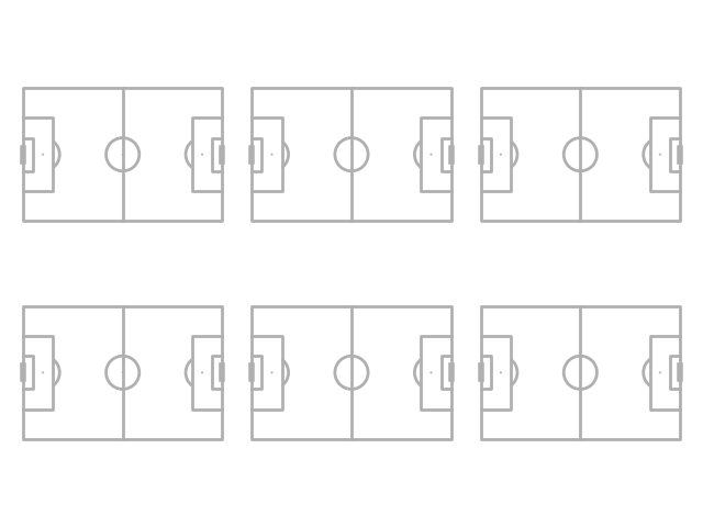
Adjusting the plot layout
mplsoccer also plots on grids by specifying nrows and ncols. The default is to use tight_layout. See: https://matplotlib.org/stable/tutorials/intermediate/tight_layout_guide.html.
pitch = Pitch()
fig, axs = pitch.draw(nrows=2, ncols=3)
But you can also use constrained layout
by setting constrained_layout=True and tight_layout=False, which may look better.
See: https://matplotlib.org/stable/tutorials/intermediate/constrainedlayout_guide.html.
pitch = Pitch()
fig, axs = pitch.draw(nrows=2, ncols=3, tight_layout=False, constrained_layout=True)

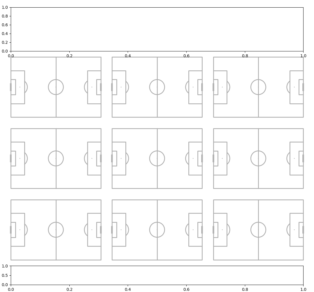
If you want more control over how pitches are placed you can use the grid method. This also works for one pitch (nrows=1 and ncols=1). It also plots axes for an endnote and title (see the plot_grid example for more information).
pitch = Pitch()
fig, axs = pitch.grid(nrows=3, ncols=3, figheight=10,
                      # the grid takes up 71.5% of the figure height
                      grid_height=0.715,
                      # 5% of grid_height is reserved for space between axes
                      space=0.05,
                      # centers the grid horizontally / vertically
                      left=None, bottom=None)
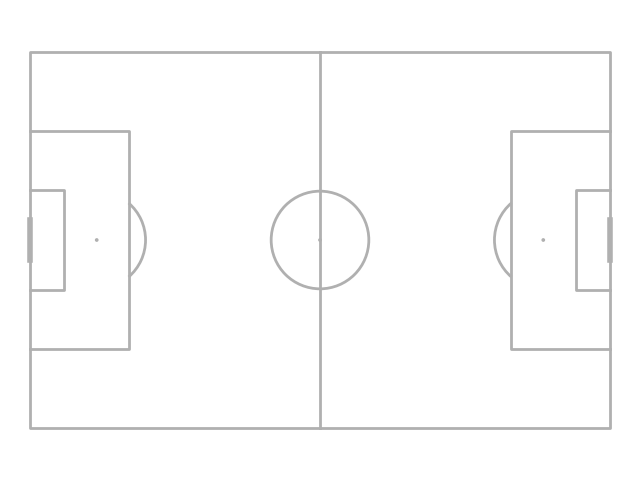
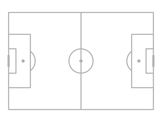
Pitch orientation
There are four basic pitch orientations. To get vertical pitches use the VerticalPitch class. To get half pitches use the half=True argument.
Horizontal full
pitch = Pitch(half=False)
fig, ax = pitch.draw()

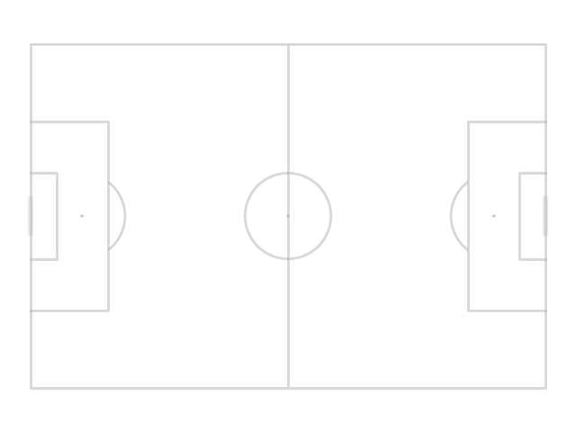
Vertical full
pitch = VerticalPitch(half=False)
fig, ax = pitch.draw()

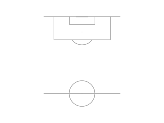
Horizontal half
pitch = Pitch(half=True)
fig, ax = pitch.draw()

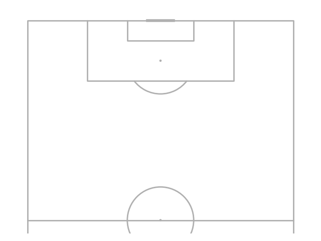
Vertical half
pitch = VerticalPitch(half=True)
fig, ax = pitch.draw()
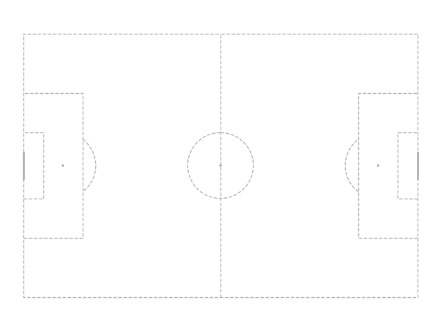
You can also adjust the pitch orientations with the pad_left, pad_right,
pad_bottom and pad_top arguments to make arbitrary pitch shapes.
pitch = VerticalPitch(half=True,
                      pad_left=-10,  # bring the left axis in 10 data units (reduce the size)
                      pad_right=-10,  # bring the right axis in 10 data units (reduce the size)
                      pad_top=10,  # extend the top axis 10 data units
                      pad_bottom=20)  # extend the bottom axis 20 data units
fig, ax = pitch.draw()
Pitch appearance
The pitch appearance is adjustable.
Use pitch_color and line_color, and stripe_color (if stripe=True)
to adjust the colors.
pitch = Pitch(pitch_color='#aabb97', line_color='white',
              stripe_color='#c2d59d', stripe=True)  # optional stripes
fig, ax = pitch.draw()

Line style
The pitch line style is adjustable.
Use linestyle and goal_linestyle to adjust the colors.
pitch = Pitch(linestyle='--', linewidth=1, goal_linestyle='-')
fig, ax = pitch.draw()
Line alpha
The pitch transparency is adjustable.
Use pitch_alpha and goal_alpha to adjust the colors.
pitch = Pitch(line_alpha=0.5, goal_alpha=0.3)
fig, ax = pitch.draw()
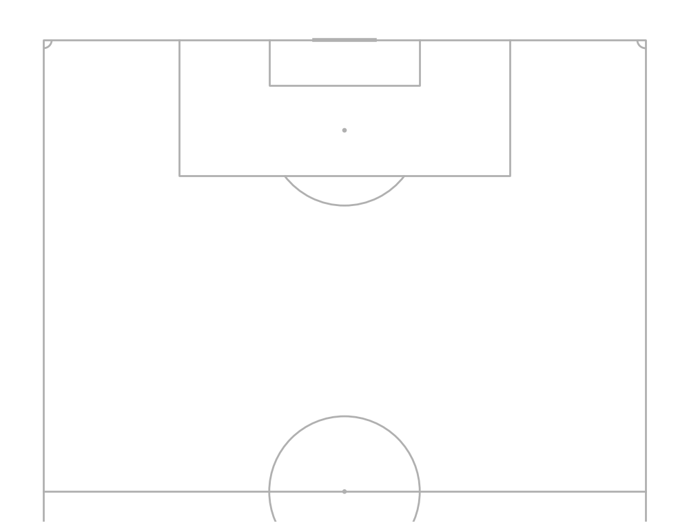
Corner arcs
You can add corner arcs to the pitch by setting corner_arcs = True
pitch = VerticalPitch(corner_arcs=True, half=True)
fig, ax = pitch.draw(figsize=(10, 7.727))
Juego de Posición
You can add the Juego de Posición pitch lines and shade the middle third
pitch = Pitch(positional=True, shade_middle=True, positional_color='#eadddd', shade_color='#f2f2f2')
fig, ax = pitch.draw()

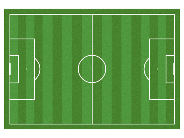
mplsoccer can also plot grass pitches by setting pitch_color='grass'.
pitch = Pitch(pitch_color='grass', line_color='white',
              stripe=True)  # optional stripes
fig, ax = pitch.draw()
Three goal types are included goal_type='line', goal_type='box',
and goal_type='circle'
fig, axs = plt.subplots(nrows=3, figsize=(10, 18))
pitch = Pitch(goal_type='box', goal_alpha=1)  # you can also adjust the transparency (alpha)
pitch.draw(axs[0])
pitch = Pitch(goal_type='line')
pitch.draw(axs[1])
pitch = Pitch(goal_type='circle', linewidth=1)
pitch.draw(axs[2])

The line markings and spot size can be adjusted via linewidth and spot_scale.
Spot scale also adjusts the size of the circle goal posts.
pitch = Pitch(linewidth=3,
              # the size of the penalty and center spots relative to the pitch_length
              spot_scale=0.01)
fig, ax = pitch.draw()
If you need to lift the pitch markings above other elements of the chart.
You can do this via line_zorder, stripe_zorder,
positional_zorder, and shade_zorder.
pitch = Pitch(line_zorder=2)  # e.g. useful if you want to plot pitch lines over heatmaps
fig, ax = pitch.draw()
Axis
By default mplsoccer turns of the axis (border), ticks, and labels.
You can use them by setting the axis, label and tick arguments.
pitch = Pitch(axis=True, label=True, tick=True)
fig, ax = pitch.draw()

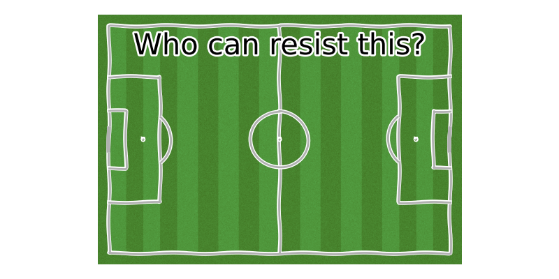
xkcd
Finally let’s use matplotlib’s xkcd theme.
plt.xkcd()
pitch = Pitch(pitch_color='grass', stripe=True)
fig, ax = pitch.draw(figsize=(8, 4))
annotation = ax.annotate('Who can resist this?', (60, 10), fontsize=30, ha='center')

plt.show()  # If you are using a Jupyter notebook you do not need this line
Total running time of the script: ( 0 minutes 5.746 seconds)